We have all been there. You spend hours crafting a complex Google Earth Engine (GEE) script to analyze vegetation health or land cover changes. You carefully filter your collections, apply your reducers, and hit "Run." The result? A flat, colorful blob on a map.
Technically, it is accurate. But does it tell a story?
In the evolving world of geospatial engineering, the ability to process data is only half the battle. The other half is presentation. Whether you are delivering a report to a non-technical stakeholder, presenting findings to a client, or simply exploring a dataset yourself, the user experience (UX) of your map matters. A static, flat map requires the viewer to trust you; an interactive, textured dashboard invites the viewer to verify your work.
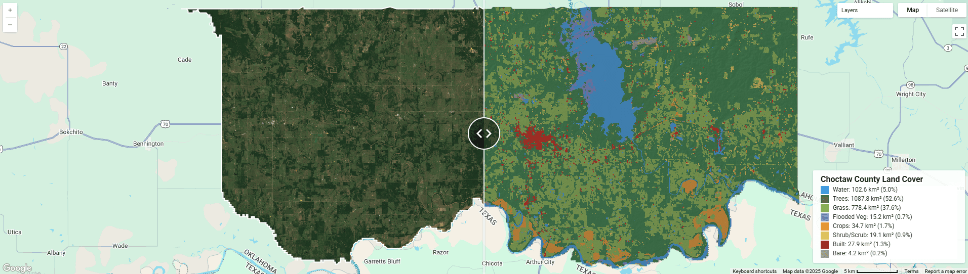
Today, we are going to bridge the gap between raw analysis and professional application development. We will walk through the creation of a "Cinematic" Land Cover Split-Viewer focusing on Choctaw County, Oklahoma, during the Spring bloom of 2025.
This isn't just a copy-paste tutorial. We are going to deconstruct three advanced concepts that will elevate your Earth Engine skills:
- Cinematic Visualization: How to blend hillshade models with classification data to add 3D depth and topographic context.
- The Split-Panel Architecture: How to use ui.SplitPanel and ui.Map.Linker to create seamless comparison tools.
- Asynchronous Statistics: How to use evaluate() to calculate server-side statistics without freezing the client-side browser.
Let’s dive into the build.
Part 1: The Data Strategy
Before we touch the user interface, we need to ensure our foundational data is pristine. For this application, we are comparing "Reality" (Optical Imagery) against "Interpretation" (AI Classification).
The Reality Layer: Sentinel-2 Harmonized
For our visual reference, we are using the Sentinel-2 Level-2A collection. However, experienced GEE users know that you should specifically use COPERNICUS/S2_SR_HARMONIZED.
Why "Harmonized"? In early 2022, the European Space Agency (ESA) changed the processing baseline for Sentinel-2, which shifted the digital numbers (DN) by a fixed offset. If you mix imagery from before and after this change without correction, your mosaics will look patchy. The Harmonized collection handles this offset automatically, ensuring consistent reflectance values across years.
In our script, we apply a standard cloud masking function using the QA60 band. This band contains bitmask information telling us which pixels are opaque clouds or cirrus clouds. By performing a bitwise operation, we strip these pixels out.
Finally, we use a .median() reducer over our date range (April 1, 2025 – June 30, 2025). Why median? A median reducer is excellent for removing outliers. If a pixel is bright white (cloud) in one image and dark green (forest) in five others, the median value will be the green forest. It is a simple, statistically robust way to generate a "clean" image for the season.
The Interpretation Layer: Dynamic World
For the land cover classification, we are using Google’s Dynamic World dataset. This is a near real-time, 10-meter resolution land cover product generated using deep learning on Sentinel-2 imagery.
Unlike Sentinel-2, land cover data is categorical. A pixel is either "Water" (0) or "Trees" (1); it cannot be 0.5. Therefore, we cannot use a .median() reducer. Instead, we use the .mode() reducer.
The Mode reducer looks at the stack of images over our three-month Spring window and asks: "What class appeared most frequently for this pixel?" If a pixel was classified as "Water" 80% of the time and "Bare Ground" 20% of the time (perhaps due to a drought or bad classification), the Mode will return "Water." This effectively smooths out temporal noise and provides a stable classification map.
Part 2: The "Cinematic" Visualization
Standard land cover maps often look like cartoons—flat patches of solid color. While this is useful for calculation, it lacks context. Does that patch of forest sit on a flat wetland or a steep mountain ridge?
To fix this, we use Hillshade Blending.
This technique borrows from cartography. We take the NASADEM digital elevation model (DEM) and generate a hillshade layer—a grayscale image simulating how sunlight hits the terrain (typically from the Northwest).
In Earth Engine, we can blend these layers mathematically using the .blend() function.
// 1. Get Elevation
var elevation = ee.Image('NASA/NASADEM_HGT/001').select('elevation');

// 2. Create Hillshade (Exaggerated height by 2x for dramatic effect)
var hillshade = ee.Terrain.hillshade(elevation.multiply(2), 315, 35).clip(choctaw);

// 3. Blend
var dwTextured = dwRgb.blend(hillshade.multiply(0.4).visualize({
    min: 0,
    max: 255,
    opacity: 0.3
}));
In the code above, we set the opacity of the hillshade to 0.3 (30%). This allows the land cover colors to remain dominant while the shadows of the terrain "bake" into the image. The result is a map that feels tactile and 3D, allowing the viewer to intuitively understand the relationship between the landscape's shape and its vegetation.
Part 3: The User Interface Architecture
Now that our data looks good, we need to build the "app" portion of the script. Earth Engine's ui module is powerful because it allows us to break out of the standard single-map paradigm.
The Split Panel
The core feature of this viewer is the ui.SplitPanel. This widget takes two standard map objects (leftMap and rightMap) and places them side-by-side with a movable handle in the middle.
However, creating two maps introduces a problem: synchronization. If you zoom in on the satellite image on the left, the land cover map on the right stays zoomed out, breaking the comparison.
To solve this, we use the Linker:
var linker = ui.Map.Linker([leftMap, rightMap]);This single line of code binds the viewport state of both maps. A pan on one is a pan on the other. This is critical for validation workflows, where an analyst needs to scrub back and forth to see if the AI model correctly identified a specific field or river bend.
Part 4: The Computation (Client vs. Server)
This is the most technical part of the script, and the area where most developers struggle. We want to display a legend that not only shows the colors but also calculates the total area of each land cover class in the current view.
To do this, we use reduceRegion to sum up the pixel area for every class in Choctaw County. This is a massive calculation involving millions of pixels.
The Trap: getInfo()
You may be tempted to try to run this calculation and retrieve the result using .getInfo(). In Earth Engine, getInfo() forces the browser (the Client) to pause and wait for the Google Cloud servers to finish the math. If the calculation takes 10 seconds, your browser freezes for 10 seconds. The UI becomes unresponsive, obviously this isn't necessarily ideal.
The Solution: evaluate()
The professional approach, which we use in this script, is Asynchronous Execution via the .evaluate() method.
stats.get('groups').evaluate(function(groups) {
  // This function runs ONLY when the server is finished.
});
When the script runs, the map loads immediately. In the background, invisible to the user, a request is sent to Google's servers to calculate the area stats. The user can pan and zoom freely. Once the server finishes the math, it "calls back" to the browser with the data, and the legend populates dynamically.
Part 5: The Complete Script
Here is the full, consolidated script. It includes the data processing, the hillshade visualization, the split-panel logic, and the asynchronous statistical calculation.
You can copy and paste this directly into the Google Earth Engine Code Editor.
// ================================================================
// Choctaw County, OK – Cinematic Split Viewer & Analyzer
// ================================================================

// 1. REGION OF INTEREST
// We filter down to Choctaw County, Oklahoma using the FAO GAUL dataset.
var choctaw = ee.FeatureCollection('FAO/GAUL_SIMPLIFIED_500m/2015/level2')
  .filter(ee.Filter.eq('ADM2_NAME', 'Choctaw'))
  .filter(ee.Filter.eq('ADM1_NAME', 'Oklahoma'));

Map.centerObject(choctaw, 10);

// 2. DATA ACQUISITION (Spring 2025)
// Focusing on the peak green-up period for the region.
var startDate = '2025-04-01';
var endDate = '2025-06-30';

// -- Sentinel-2 (Mosaicked for full coverage) --
function maskS2clouds(image) {
  var qa = image.select('QA60');
  var cloudBitMask = 1 << 10;
  var cirrusBitMask = 1 << 11;
  var mask = qa.bitwiseAnd(cloudBitMask).eq(0)
      .and(qa.bitwiseAnd(cirrusBitMask).eq(0));
  return image.updateMask(mask).divide(10000);
}

var s2 = ee.ImageCollection('COPERNICUS/S2_SR_HARMONIZED')
  .filterBounds(choctaw)
  .filterDate(startDate, endDate)
  .filter(ee.Filter.lt('CLOUDY_PIXEL_PERCENTAGE', 20))
  .map(maskS2clouds)
  .median() // Median creates a clean mosaic, removing artifacts
  .clip(choctaw);

// -- Dynamic World (Mode mosaic to reduce noise) --
var dw = ee.ImageCollection('GOOGLE/DYNAMICWORLD/V1')
  .filterBounds(choctaw)
  .filterDate(startDate, endDate)
  .select('label')
  .mode() // Use mode to find the most common class per pixel
  .clip(choctaw);

// -- Terrain (Real Elevation for texture) --
var elevation = ee.Image('NASA/NASADEM_HGT/001').select('elevation');
var hillshade = ee.Terrain.hillshade(elevation.multiply(2), 315, 35).clip(choctaw);

// 3. VISUALIZATION

// Sentinel-2 True Color
var visParamsS2 = {
  min: 0.0,
  max: 0.3,
  bands: ['B4', 'B3', 'B2'],
  gamma: 1.2
};

// Dynamic World Palette
var dwPalette = [
  '#419bdf', // Water
  '#397d49', // Trees
  '#88b053', // Grass
  '#7a87c6', // Flooded Veg
  '#e49635', // Crops
  '#dfc35a', // Shrub/Scrub
  '#c4281b', // Built
  '#a59b8f', // Bare
  '#b39fe1'  // Snow/Ice
];

var dwVis = {min: 0, max: 8, palette: dwPalette};

// Composite: Blend Land Cover with Hillshade for "3D" look
var dwRgb = dw.visualize(dwVis);
var dwTextured = dwRgb.blend(hillshade.multiply(0.4).visualize({
    min: 0,
    max: 255,
    opacity: 0.3 // Subtle terrain texture
}));

// 4. UI CONSTRUCTION: SPLIT PANEL

// Create two maps
var leftMap = ui.Map();
var rightMap = ui.Map();

// Link them so they zoom/pan together
var linker = ui.Map.Linker([leftMap, rightMap]);

// Add layers
leftMap.addLayer(s2, visParamsS2, 'Sentinel-2 Natural');
leftMap.addLayer(ee.FeatureCollection(choctaw).style({color:'white', fillColor:'00000000', width: 2}), {}, 'Border');

rightMap.addLayer(dwTextured, {}, 'Land Cover (Textured)');

// Create the SplitPanel
var splitPanel = ui.SplitPanel({
  firstPanel: leftMap,
  secondPanel: rightMap,
  orientation: 'horizontal',
  wipe: true,
  style: {stretch: 'both'}
});

// Replace default UI
ui.root.widgets().reset([splitPanel]);
leftMap.centerObject(choctaw, 11);

// 5. ADDING LEGEND & STATS

var panel = ui.Panel({
  style: {
    position: 'bottom-right',
    padding: '8px 15px',
    width: '300px',
    backgroundColor: 'rgba(255, 255, 255, 0.9)'
  }
});

var title = ui.Label({
  value: 'Choctaw County Land Cover',
  style: {fontWeight: 'bold', fontSize: '16px', margin: '0 0 4px 0'}
});
panel.add(title);

var labels = ['Water', 'Trees', 'Grass', 'Flooded Veg', 'Crops', 'Shrub/Scrub', 'Built', 'Bare', 'Snow/Ice'];

// Calculate Area (Server-side aggregation)
var areaImage = ee.Image.pixelArea().addBands(dw);
var stats = areaImage.reduceRegion({
  reducer: ee.Reducer.sum().group({
    groupField: 1,
    groupName: 'class_index',
  }),
  geometry: choctaw.geometry(),
  scale: 100, // Approx scale for speed
  maxPixels: 1e10
});

// Build Legend dynamically based on computed stats
// Note: evaluate() makes the server-side numbers available to the client-side UI
stats.get('groups').evaluate(function(groups) {
  var totalArea = 0;
  var classAreas = {};

  groups.forEach(function(g) {
    classAreas[g.class_index] = g.sum;
    totalArea += g.sum;
  });

  labels.forEach(function(name, index) {
    var sqKm = (classAreas[index] || 0) / 1e6; // Convert m2 to km2
    var pct = ((classAreas[index] || 0) / totalArea) * 100;

    if (pct > 0.1) { // Only show classes present > 0.1%
        var colorBox = ui.Label({
          style: {
            backgroundColor: dwPalette[index],
            padding: '8px',
            margin: '0 8px 0 0'
          }
        });

        var description = ui.Label({
          value: name + ': ' + sqKm.toFixed(1) + ' km² (' + pct.toFixed(1) + '%)',
          style: {margin: '0 0 4px 0', fontSize: '12px'}
        });

        var row = ui.Panel({
          widgets: [colorBox, description],
          layout: ui.Panel.Layout.Flow('horizontal')
        });
        panel.add(row);
    }
  });
});

rightMap.add(panel);
Part 6: Making It Yours
The beauty of this script is its adaptability. While I hardcoded Choctaw County and Spring 2025, you can repurpose this engine for any location on Earth.
To change the location, modify the ADM2_NAME filter in the first block of code to your desired county (or use a custom geometry). The entire pipeline—cloud masking, hillshade generation, and statistical calculation—is region-agnostic. It will automatically scale to fit your new boundary.
To change the timeframe, simply adjust the startDate and endDate variables. This is particularly powerful for analyzing seasonality. You could duplicate the script, set one to Winter and one to Summer, and compare how the "Grass" and "Crop" classes fluctuate in area.
A Note for Python Developers
While the JavaScript Code Editor is unrivaled for this type of rapid UI prototyping, I know many of you prefer to work within the Python ecosystem for its data science libraries.
I have ported this exact workflow—including the split-map visualization and the area calculations—into a Python Jupyter Notebook using the geemap library. It utilizes Pandas for the statistics table, making it a great starting point for further data analysis.
[Download the Python/Colab Notebook Here]
Conclusion
In geospatial engineering, code is the tool, but insight is the product.
By moving from static GeoTIFF exports to interactive applications, you provide your users with the context they need to understand the data. The addition of hillshade blending transforms an abstract classification into a recognizable landscape. The split-panel interface invites comparison and validation. And the use of asynchronous evaluation ensures that the experience remains fluid and professional.
Take this script, break it, modify it, and use it to tell the story of your own region.
Frequently Asked Questions (FAQ)
1. Why do we use .mode() for Dynamic World but .median() for Sentinel-2?
Sentinel-2 data is continuous (reflectance values), so median() helps find the "middle" pixel value, effectively removing clouds and shadows to create a clean composite. Dynamic World data is categorical (classes 0-8, representing things like Water or Trees). You cannot calculate the "median" of a land class. Instead, we use mode() to find the class that appeared most frequently during the date range, which stabilizes the classification.
2. What does the evaluate() function actually do?
In the code, stats.get('groups').evaluate(...) is the bridge between the server and the client. It tells Earth Engine to process the statistics asynchronously on Google's servers. Once the heavy math is done, it triggers the callback function in your browser to build the legend. If you used getInfo() instead, your browser would freeze and become unresponsive while waiting for the calculation to finish.
3. How do I change the location to my own county?
You can modify line 6 of the script. Change ADM2_NAME to your county name and ADM1_NAME to your state or province. As long as the name matches the entries in the FAO GAUL dataset (which covers the globe), the map will automatically center and recalculate statistics for your new region.
4. Why is it important to use the "Harmonized" Sentinel-2 collection?
In early 2022, the European Space Agency (ESA) updated the processing baseline for Sentinel-2, which shifted the digital numbers (DN) used to represent brightness. The "Harmonized" collection (COPERNICUS/S2_SR_HARMONIZED) automatically adjusts older images to match the new baseline. If you don't use this, comparisons between pre-2022 and post-2022 imagery may look inconsistent or yield incorrect spectral analysis.
5. Can I export the statistics to a CSV file?
Yes. While this script displays the statistics on the screen for immediate feedback, you can export them for reporting. You would need to convert the stats dictionary into a Feature Collection and use Export.table.toDrive(). If you are using the Python notebook version linked above, you can simply use df.to_csv('stats.csv') via the Pandas library.